Tektronix 5 Series Mixed Signal Oscilloscope (MSO54/56/58)

Tektronix 5 Series Mixed Signal Oscilloscope (MSO54/56/58)

Core parameters and characteristics of the product

1. Basic hardware specifications

Category detailed parameters

Channel configurations MSO54 (4 channels), MSO56 (6 channels), and MSO58 (8 channels) all support FlexChannel technology, and a single channel is compatible with:

-Analog probe (TekVPI) ®  Or BNC interface)

-8-channel digital probe (TLP058 FlexChannel Logic Probe)

Bandwidth range: Basic bandwidth of 350 MHz (default), supports upgrades: 500 MHz, 1 GHz, 2 GHz (requires corresponding bandwidth options, such as SUP5-BW3T54)

Sampling performance with a maximum sampling rate of 6.25 GS/s, supporting real-time sampling, interpolation real-time sampling, and equivalent time sampling (only applicable to repetitive signals)

Record length standard 62.5 M points/channel, optional upgrade to 125 M points/channel (options 5-RL-125M/SUP5-RL-125M)

15.6-inch HD capacitive touch screen (1920 × 1080 pixels) with optimized touch operation logic, supporting multi finger gestures, double-click configuration, etc

Capture capability up to 500000 waveforms per second, FastAcq mode can reduce waveform acquisition dead time and accurately capture transient events such as spikes and short pulses

Optional integrated functions include a 50 MHz arbitrary function generator (AFG), digital multimeter (DVM), and trigger frequency counter

2. Core technological advantages

FlexChannel technology: No need to replace hardware modules, single channel can switch between analog/digital signal acquisition, flexible adaptation to mixed signal debugging scenarios.

Multidimensional triggering system: covering basic triggering, advanced triggering, and bus triggering, it can accurately capture target signal events.

Unrestricted waveform display: Supports unlimited display of mathematical waveforms, reference waveforms, and bus waveforms (limited by system memory).

TekSecure security feature: supports secure memory erasure and protects sensitive test data.

Accessories and optional features

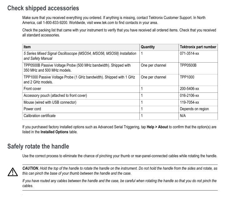
1. Standard accessories (included with the box)

Accessory Name Quantity Specification/Purpose Tektronix Model

Installation and Safety Manual 1 Instrument Installation and Safety Operation Guide 071-3514-xx

Passive voltage probe, one 350/500 MHz model per channel, equipped with TPP0500B (500 MHz bandwidth); 1/2 GHz model with TPP1000 (1 GHz bandwidth) TPP0500B, TPP1000

Front panel cover 1 protects the instrument front panel interface 200-5406-xx

Accessory bag 1 stores small accessories, attached to the front panel cover 016-2106-xx

Wired USB Mouse 1 Auxiliary Operation Interface 119-7054-xx

The voltage standard for power cord 1 to adapt to the corresponding region depends on the region

Calibration Certificate 1: Instrument Factory Calibration Certificate N/A

2. Recommended accessories (optional)

Accessory name, purpose, model/specification

Hard transport box instrument transportation protection HC5

Rack installation kit installs the instrument onto a standard equipment rack (requiring 7U space) RM5

Mini keyboard for convenient text/parameter input 119-7275-xx

GPIB-USB adapter implements GPIB interface extension TEK-USB-488

TekVPI to BNC adapter compatible with BNC probe and TekVPI interface TPA-BNC

Off ramp pulse generator assisted multi-channel off ramp calibration 067-1686-xx

High voltage differential probe for high voltage signal measurement (such as THDP0100: ± 6 kV, 100 MHz) THDP0100, THDP0200, etc

Current probe current signal measurement (such as TCP0020: 50 MHz, 20 A AC/DC) TCP0020, TCP0030A, etc

3. Core optional function options

Function Category Options Model Details Features

Arbitrary Function Generator (AFG) 5-AFG (pre installed), SUP5-AFG (upgraded) - waveform types: sine, square wave, pulse, ramp, etc. 13 preset waveforms+arbitrary waveform

-Maximum frequency: 50 MHz (sine wave)

-Maximum output amplitude: 5 Vp-p (high impedance load)

-Sampling rate: 250 MS/s, any waveform recording length of 128K samples

Advanced Jitter Analysis (DJA) 5-DJA (pre installed), SUP5-DJA (upgraded) - supports 30+industry standard jitter and eye chart measurements: TIE TJ@BER 、 DDJ、DCD、 Eye height, eye width, Q factor, etc

-Generate analysis views such as jitter summary table, bathtub curve, eye diagram, etc

Bandwidth upgrade SUP5-BW3T54 (4-channel 350 → 500 MHz), SUP5-BW3T104 (4-channel 350 → 1 GHz), SUP5-BW3T204 (4-channel 350 → 2 GHz), etc. - Partial upgrades only require a license (such as 350 → 500 MHz), while high bandwidth upgrades need to be sent back to the service center for hardware replacement

-Upgrade with calibration data and new front-end bandwidth labels

Serial bus triggering and analysis -5-SRAUDIO (audio bus), 5-SRAUTO (car bus), 5-SRCOMP (computer bus), 5-SRENET (Ethernet), 5-SREMBD (embedded bus), 5-SRUSB2 (USB 2.0) - supports buses: I2S, LJ, RJ, TDM (audio); CAN, LIN, FlexRay (automotive); RS-232/422/485/UART (computer); 10BASE-T/100BASE-T (Ethernet); I2C, SPI (embedded); USB 2.0 LS/FS/HS

Record length upgrade 5-RL-125M (pre installed), SUP5-RL-125M (upgraded) will increase the default 62.5M point/channel record length to 125M point/channel, which can capture more waveform data points

Service options T3 (3-year warranty), T5 (5-year warranty), C3 (3-year calibration), C5 (5-year calibration) - warranty includes parts, labor, and domestic transportation within 2 days

-Calibration includes traceable verification reports, covering initial calibration and subsequent annual calibration

Instrument installation and basic configuration

1. Preparation before installation and environmental requirements

(1) Accessory inspection

After unpacking, it is necessary to verify all items against the packing list, including the host, standard accessories, and selected option modules/probes, to confirm that there are no missing or damaged items.

(2) Environmental and power requirements

Category requirements details

The working temperature is 0 ° C~+50 ° C (+32 ° F~+122 ° F), and at least 2 inches (51 mm) of ventilation space should be reserved on both sides and the rear of the instrument

Working humidity 5%~90% relative humidity (≤ 40 ° C); 5%~55% relative humidity (>40 ° C~50 ° C), no condensation

Working altitude up to 3000 meters (9842 feet)

Power specification voltage: 100 V~240 V AC RMS (± 10%), single-phase

Frequency: 50/60 Hz (90 V~264 V), 400 Hz (103 V~127 V)

Maximum power consumption: 400 W (all models)

2. Key configuration steps

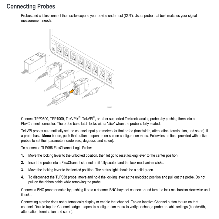
(1) Probe connection and compensation

Probe compensation is the core step to ensure measurement accuracy. Taking the TPP0500B/TPP1000 passive probe as an example:

Connect probe: Insert the probe into the FlexChannel connector and hear a "click" sound to indicate it is locked in place. The TekVPI probe will automatically configure channel parameters (bandwidth, attenuation, etc.).

Connect compensation signal: Connect the probe tip to the 1 kHz square wave source (lower terminal) of the instrument front panel "PROBE COMP", connect the probe ground clamp to the ground terminal (upper terminal), and remove the probe tip accessory to ensure good contact.

Display Square Wave: Press the "Autoset" button on the front panel, and the screen will display a stable 1 kHz square wave.

Perform compensation: double-click the channel badge (such as Ch1) → open the "Probe Setup" panel → click on "Compensate Probe", wait for compensation to complete, and the status bar will display "Pass" to indicate success (if "Fail" is displayed, the probe needs to be reconnected and the operation repeated).

(2) Signal Path Compensation (SPC)

SPC is used to correct DC deviations in internal signal paths caused by temperature changes or long-term drift. It is recommended to:

Execute when the ambient temperature changes by more than 5 ° C (41 ° F);

Execute once a week (if the commonly used vertical scale is ≤ 5 mV/div).

Operation steps:

Disconnect all probes, cables, and external signal inputs;

Preheat the instrument for at least 20 minutes when powered on;

Select "Utility>Calibration>Run SPC" from the top menu bar;

Wait for the compensation to be completed (several minutes per channel), and the status bar will display "SPC Pass". If it fails, record the error message and contact the support team.

(3) Network and Remote Access Configuration

Physical connection: Connect the instrument LAN port to the network switch/router using CAT5 Ethernet cable;

Network settings:

Select "Utility>I/O>LAN";

Automatic IP acquisition (default): Select "Auto", and the instrument obtains the IP address, subnet mask, and gateway through DHCP;

Manual settings: Select "Manual" and enter the static IP, subnet mask, and DNS address provided by the IT department;

Connection verification: Click on "Test Connection", the LAN status icon turns green to indicate successful connection;

Remote access: Enter the instrument IP address in a PC browser on the same network and select "Instrument Control (e * Scope ®)”， The instrument can be remotely operated through a browser (supporting mouse control of all interface functions).

(4) Channel skew (Desk view)

When measuring multi-channel timing, it is necessary to correct the propagation delay difference between probes, and two methods are supported:

Quick visual method:

Connect all probes to the "PROBE COMP" signal and activate the corresponding channel;

Double click on the waveform view and set "Waveform Mode" to "Overlay";

Adjust the horizontal scale to clearly display channel delay differences;

Double click on the target channel badge ->"Other" ->"Deskew", adjust with the multifunction knob to align the waveform edge with the reference channel.

Measurement method:

Add "Delay" measurement ("Add New... Measure>Timing>Delay");

Set the reference channel as Source 1 and the target channel as Source 2;

Adjust the Desk value of the target channel to minimize measurement delay.

Detailed explanation of core operations and functions

1. Signal acquisition and triggering system

(1) Fast waveform display (Autoset)

Press the "Autoset" button on the front panel, and the instrument will automatically complete the following operations:

Analyze the signal characteristics of the lowest numbered display channel (analog/digital);

Adjust horizontal (time base), vertical (scale, position), and trigger parameters;

Stable display waveform (optimizing the vertical scale of all active waveforms in stacking mode and evenly distributing waveforms in stacking mode).

Note: AutoSet ignores mathematics, reference, and bus waveforms, and signals with frequencies<40 Hz will be judged as "no signal".

(2) Collection mode selection

By double clicking the "Acquisition" badge, the following modes can be selected:

Applicable scenario characteristics of the mode

Sample: Conventional signal acquisition retains the first sample of each acquisition interval without post-processing

Peak Detection captures high-frequency spikes and alternates between narrow pulses to preserve the highest/lowest samples of adjacent acquisition intervals

High Res high-precision measurement, low-noise scene based on sampling rate FIR filtering, suppresses aliasing, ensures ≥ 12 bit vertical resolution, supports FastAcq

Envelope observes the range of signal changes, captures the extreme values of multiple collected signals, and displays the envelope waveform

Average reduces the average waveform of random noise collected multiple times, and the average frequency can be set

FastAcq captures transient events to reduce acquisition dead time, supports intensity display (reflecting signal frequency), and can choose color palettes such as "Temperature" and "Spectral"

(3) Trigger type and configuration

Trigger is used to define when to start collecting waveforms. The 5 series supports a variety of trigger types, including:

Edge trigger (basic):

Trigger source: any analog/digital channel, mathematical/reference waveform;

Slope: rising edge, falling edge, arbitrary edge;

Level: Double click the "Level" knob to set it, or press the knob to automatically set it to 50% of the signal peak to peak value;

Coupling: DC (transmitting all signals), HF Reject (attenuation>50 kHz signals), LF Reject (attenuation<50 kHz signals), Noise Reject (increasing hysteresis, anti noise).

Pulse width trigger:

Trigger conditions: Pulse width<,>,=, ≠ set value, or within/outside the specified range;

Polarity: positive pulse, negative pulse, any polarity;

Application scenario: Narrow pulse and wide pulse fault detection in digital logic.

Bus trigger:

Prerequisite: Corresponding buses (such as CAN, I2C) have been added;

Configuration steps:

Click on "Add New Bus" → select the bus type (such as CAN);

Set bus parameters (such as CAN baud rate, signal source, threshold);

Double click the "Trigger" badge ->select "Trigger Type>Bus" ->select the trigger bus (such as Bus1);

Set triggering conditions (such as CAN ID, data bytes, frame type).

Timing trigger (A&B events):

Function: After triggering event A, data collection will only be initiated upon detecting event B;

to configure:

Select 'Trigger Type>Sequence';

Configure event A (such as Ch1 rising edge);

Configure event B (such as Ch2 pulse width>100 ns);

Set trigger logic: trigger the first B event (with a delay time that can be set), or the Nth B event.

2. Measurement and analysis functions

(1) Basic measurement operation

Add measurement: Click on "Add New... Measure" in the results bar ->select the measurement source (such as Ch1) ->select the measurement category (amplitude, timing, jitter, etc.) ->double-click the measurement item (such as "Peak to Peak"), and the measurement badge will be automatically added to the results bar.

Measurement configuration: Double click the measurement badge → Open the configuration menu, you can:

Label (for easy identification, such as "VCC peak to peak value");

Set reference level (such as 10% -90% rise time threshold);

Enable statistical display (mean, minimum, maximum, sample size);

Set measurement gating (only measure specific areas of the waveform, such as between the cursor and the screen display area).

(2) Core measurement categories and parameters

Application scenarios of key measurement items in measurement categories

Peak to peak value, maximum value, minimum value of amplitude measurement AC RMS、DC、 Analysis of positive/negative overshoot, top, bottom, and area voltage/amplitude characteristics (such as power ripple, signal amplitude consistency)

Timing measurement of frequency, cycle, rise/fall time, pulse width, duty cycle, delay, phase, data rate, and verification of unit interval signal timing characteristics (such as clock frequency, signal delay, duty cycle deviation)

Jitter measurement (basic) time interval error (TIE) preliminary jitter detection

Jitter Measurement (Advanced, requires DJA option) Deterministic Jitter (DJ), Random Jitter (RJ), Total Jitter（ TJ@BER ）Data related jitter (DDJ), periodic jitter (PJ), high-speed serial signal (such as USB, Ethernet) jitter compliance testing

Eye diagram measurement (DJA option required) eye height, eye width, eye height @ BER, eye width @ BER, Q-factor high-speed signal integrity assessment (such as SerDes, DDR)

(3) Bus decoding and analysis

Taking CAN bus as an example (requires 5-SRAUTO/SUP5-AFG options):

Add CAN bus:

Click on "Add New Bus" → select "Bus Type>CAN";

Set "Source" (channel connected to CAN_SH), "Threshold" (logic high level, such as 1.4 V), "Bit Rate" (such as 500 kbps), and "Identifier Format" (standard 11 bits/extended 29 bits);

Decoding display: The bus waveform is automatically displayed, and the decoding result is superimposed on the waveform (such as ID=0x123, Data=0x01 0x02);

Add bus result table: Click on the results bar "Results Table>Bus Decoder" to generate a table containing ID, data, frame type, and timestamp, which can be saved as a. csv file.

(4) Waveform Analysis View

In addition to conventional waveform display, it supports multiple analysis views:

Histogram: Display the distribution of measurement values (such as amplitude distribution, jitter distribution), double-click the measurement badge → click "Histogram" to add;

Spectrum: Display the frequency components of the signal. Double click the measurement badge ->click "Spectrum" to set the FFT window (rectangle, Hanning, Hamming, etc.);

Eye Diagram: To select the DJA option, double-click on the jitter measurement badge and then click on "Eye Diagram" to configure the eye diagram template and BER threshold;

Time Trend: Display the change of measurement values over time (such as long-term drift of power supply voltage), double-click the measurement badge → click "Time Trend".

3. Display and operation optimization

(1) Waveform display mode

Stacking mode (default): Each waveform is vertically stacked in independent "slices", with independent vertical scales for easy observation of multi-channel signals;

Overlay mode: All waveforms are stacked in the same grid for easy comparison of waveform shapes (such as reference waveforms and measured waveforms);

Switching method: Double click on the blank area of the waveform view ->click on "Display Mode" to switch.

(2) Zoom and cursor operation

Zoom mode enabled:

Press the "Zoom" button on the front panel;

Click on the "Draw-a-Box" in the results bar, drag and draw the area of interest on the waveform (automatically enters zoom mode);

Double click the "Zoom" icon in the upper right corner of the waveform view.

Zoom operation:

Zoom knob (middle): Adjust the size of the zoom box (zoom in/out);

Translation knob (outer side): Move the zoom box position (left and right translation);

Cursor measurement:

Press the "Cursors" button on the front panel, or click on "Add New... Cursors" in the results bar;

Use the multifunctional knobs A/B to move the cursor, supporting waveform cursor (measuring amplitude+time), vertical cursor (measuring time difference), and horizontal cursor (measuring amplitude difference);

Double click cursor reading → configurable cursor type and source (supports cross channel comparison).

4. Data storage and recall

(1) Can store data types and formats

Data Type Storage Format Usage

Screenshot in PNG, BMP, JPG format to save the current interface (including menu, waveform, measurement results) for document reporting

Waveform data. wfm (Tektronix specific),. csv (universal format) to save channel, mathematical, and reference waveform data for subsequent analysis or sharing

Instrument settings. set saves all channel, trigger, measurement, and display settings for easy repetition of testing scenarios

Report PDF, single file webpage containing measurement results, waveform screenshots, instrument configuration, annotations, supports adding custom notes

Conversation. tss (compressed file) saves settings and all waveform data for offline analysis or transfer of testing tasks

(2) Storage operation steps (taking saving waveforms as an example)

Select "File>Save As>Waveform";

Configure storage parameters:

Save location: Select a USB drive (such as E:, F:) or internal storage (C:), click "Browse" to navigate to the folder;

File name: default "Tek000", modifiable (supports Chinese/English), enable "Auto Increment File Name" to automatically increment numbers (such as Tek001, Tek002);

Save type: Choose. wfm (to preserve complete information) or. csv (to facilitate Excel analysis);

Save source: Select "All" (all active waveforms) or a single waveform (such as Ch1, Math1);

Click "OK" to save, and after successful saving, the status bar will display a confirmation message.

(3) Quick storage (User key)

First use: Press the "User" button on the front panel → open the "Save As" menu, configure the storage type (such as waveform), position, and format, and click "OK";

Subsequent use: Press the "User" button again to automatically save data according to the previous configuration (no need to repeat the settings).

(4) Data recall operation (taking the recall reference waveform as an example)

Click on 'Add New Ref' (settings bar);

Select storage location (such as USB drive) and file type (. wfm);

Select the target waveform file, click "Recall", and add the reference waveform (Rx) to the waveform view for comparative analysis.

Common problems and precautions

1. Safety precautions

ESD protection: When operating the probe or DUT, wear a grounded anti-static wristband (grounding terminal provided on the instrument front panel) to avoid touching the probe tip or instrument input interface;

Input voltage limit: When the analog channel is set to 1 M Ω, the maximum input is 300 VRMS, and when set to 50 Ω, the maximum input is 5 VRMS. Exceeding this limit may damage the instrument;

Power safety: Only use power cords that come with the box or are Tektronix certified, ensure good grounding, and avoid use in humid environments.

2. Common troubleshooting

Troubleshooting steps for fault phenomena

No waveform display. 1. Check if the probe connection is locked; 2. Confirm that the channel is enabled (click the "Inactive Channel" button in the settings bar); 3. Press the "Autoset" button; 4. Check if the trigger source is correct and if the trigger mode is "Auto"

Inaccurate measurement results: 1. Perform probe compensation; 2. Run SPC; 3. Check the reference level setting; 4. Confirm that there is no signal clipping (the channel badge displays "Clipping" and the vertical scale needs to be adjusted)

Network connection failure: 1. Check the network cable connection; 2. Confirm that the router/DHCP service is functioning properly; 3. Manually set static IP testing; 4. Restart the instrument and router

Option cannot be enabled. 1. Confirm that the license has been installed ("Help>About"); 2. Restart the oscilloscope; 3. Check if the license file corresponds to the instrument serial number