Tektronix XYZs of Oscilloscopes



Tektronix XYZ oscilloscope

Overview

The XYZs of Oscilloscopes Primer launched by Tektronix aims to help engineers, technicians, educators, and others master the basic knowledge and operation of oscilloscopes, without the need for prior mathematical or electronic knowledge. Through theoretical explanations, chart examples, exercises, and terminology lists, it covers the entire process of oscilloscopes from principle to practice, ultimately allowing readers to describe the working principle of oscilloscopes, distinguish oscilloscope types, understand waveforms and controls, and complete basic measurements.

Signal Integrity

Core significance: The ability of oscilloscope systems to accurately reconstruct waveforms, analogous to the "imaging accuracy" and "clarity" of cameras, directly affects the time to market cycle of electronic design, product reliability, EMI compliance, and probe can also affect the signal integrity of measurement systems.

Root cause of the problem:

Speed improvement: The processor clock speed reaches 2-5GS/s, the DDR3 memory clock exceeds 2GHz, the rise time is 35ps, and the high-speed characteristics penetrate into fields such as automotive and consumer electronics, with most designs becoming "high-speed designs".

Physical limitations: The propagation time of the circuit board bus has remained unchanged for decades, and 6-inch traces become transmission lines when the signal rise time is less than 4-6ns, causing crosstalk, ground bounce, and EMI rise.

Model failure: When the signal edge velocity is 4-6 times or more the signal path delay, the lumped circuit model is no longer applicable.

Solution: Digital errors often stem from simulation problems, and it is necessary to use an oscilloscope to observe waveform details, transient signals, and correlate high-speed waveforms with data patterns.

‍

Principle and waveform of oscilloscope (The Oscilloscope)

(1) Working principle

Oscilloscope is a graphical display device that converts electrical signals into a "time voltage" graph

X-axis (horizontal): Time

Y-axis (vertical): voltage

Z-axis (brightness): Display intensity (represented by color grading in DPO to indicate signal frequency)

(2) Waveform types and characteristics

Application scenarios of key characteristics of waveform types

Sine wave mathematical harmony, AC power supply, signal generator output basic test signal, power supply voltage

Square wave/rectangular wave square wave high and low level time are equal, rectangular wave unequal amplifier testing, timing signal (TV/computer)

Linear variation of sawtooth/triangular wave voltage (ramp) simulation oscilloscope horizontal scanning, TV grating scanning

Step/pulse step is a sudden voltage change, pulse is an "on-off" change power switch, computer data transmission (1-bit information), radar

Periodic/non periodic periodic periodic signal repetition, non periodic signal continuous change periodicity: sine wave; Non periodic: transient faults

Synchronous/asynchronous synchronous signals have a timing relationship (such as clock and data), asynchronous signals have no (such as keyboard and computer clock). Synchronization: internal signals of the computer; Asynchronous: Peripheral interaction

Complex waves combined with multiple waveform features, including amplitude/phase/frequency variation composite video signals and communication eye diagrams (such as 622Mb/s serial data)

(3) Waveform measurement indicators

Frequency and Period: Frequency (Hz)=1/Period (seconds), for example: A 3Hz sine wave has a period of 1/3 second.

Voltage: Peak to Peak Value (Vp-p, signal maximum to minimum voltage difference), Peak Value (Vp, ground to maximum voltage).

Amplitude: usually refers to the maximum voltage from ground to the signal. For example, a waveform with an amplitude of 1V has a peak to peak value of 2V.

Phase: Sine wave 1 cycle=360 °, phase difference refers to the timing difference between two similar signals, for example: current and voltage differ by 90 ° (1/4 cycle).

Automatic measurement of digital oscilloscope: including cycle, duty cycle, frequency, delay, maximum/minimum value, rise/fall time, overshoot RMS、 Shake, etc.

Types of Oscilloscopes

Type Core Architecture Key Features Applicable Scenarios

Digital Storage Oscilloscope (DSO) serial processing (amplification → ADC → storage → microprocessor → display) stores transient signals, permanently saves and processes them, without real-time brightness grading, low-speed repetition or single high-speed multi-channel design (such as capturing glitches)

Digital Fluorescence Oscilloscope (DPO) parallel processing (amplification → ADC → digital fluorescence database → direct display, microprocessor parallel processing) real-time 3D display (time, amplitude, amplitude distribution), high waveform capture rate (million level/second), general design and troubleshooting of analog oscilloscope display characteristics (video signal, communication mask testing)

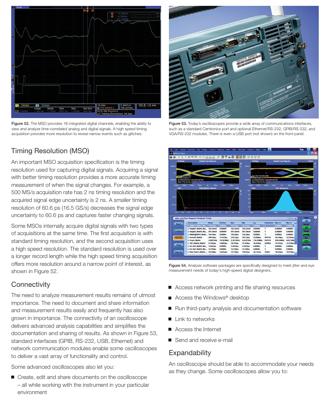
Mixed domain oscilloscope (MDO) combined with RF spectrum analyzer+MSO/DPO to correlate digital, analog, and RF signal time, reducing measurement uncertainty of cross domain events. Embedded RF design (such as Zigbee radio, observing command and RF event delay)

Mixed signal oscilloscope (MSO) combined with DPO performance and 16 channel logic analyzer to simultaneously observe analog and digital signals, supporting protocol decoding (I2C/CAN, etc.) and digital circuit debugging (verifying the correlation between logic state and analog waveform)

Digital sampling oscilloscope first samples and then amplifies (sampling bridge → amplification) with high bandwidth (up to 80GHz), limited dynamic range (1Vp-p), safe input voltage of 3V, measurement frequency exceeding the oscilloscope sampling rate for repetitive signals (such as high-speed timing)

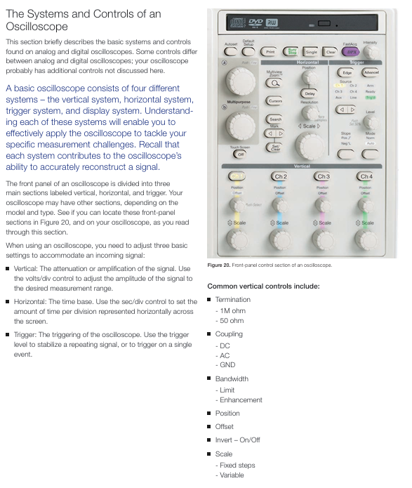
Oscilloscope Systems and Controls

(1) Vertical System and Control

Core functions: Adjust the vertical position and scaling of waveforms, set signal coupling and bandwidth.

Key controls:

Position and volts/div: volts/div is the scaling factor, for example: 5V/div x 8 vertical partition=40V maximum display voltage; Combined with probe attenuation (10X probe needs to be divided by 10).

Input coupling: DC (display full signal), AC (block DC, center signal), GND (disconnect input, display 0V line).

Bandwidth limitation/enhancement: Bandwidth limitation reduces noise, while bandwidth enhancement (DSP filtering) expands bandwidth and improves phase linearity.

(2) Horizontal System and Control

Core function: Control signal acquisition (sampling mode, sampling rate) and waveform horizontal position, scaling.

Key controls and concepts:

Sampling mode:

Sampling mode: 1 sampling point=1 waveform point.

Peak detection mode: Save the maximum/minimum values within 2 waveform intervals to capture fast transients (such as narrow pulses).

High resolution (Hi Res) mode: averaging multiple sampling points to reduce noise, suitable for a single event.

Envelope mode: displays the range of signal variation based on the maximum/minimum values collected multiple times.

Average mode: Average the waveform points collected multiple times, reduce noise, and repeat the signal.

Sampling method:

Real time sampling: Collect enough points in one scan, suitable for signals with a frequency<1/2 of the oscilloscope's maximum sampling rate, and the only method to capture a single transient.

Equivalent time sampling: Multiple scans capture repeated signal segments (random: sampling clock is asynchronous with trigger, supports pre trigger; sequential: delay increment Δ t per trigger, high time resolution), suitable for frequency oversampling rate of repeated signals.

Position and Sec/div: Sec/div is the time base, for example: 1ms/div x 10 horizontal partitions=10ms total display time.

Other: Time base selection (main time base/delay time base), scaling/shifting, searching (finding specific events), XY mode (X-axis is the signal rather than time, measuring phase difference).

(3) Trigger system and control

Core function: Synchronize horizontal scanning, stabilize repetitive waveforms or capture single waveforms.

Key controls and types:

Trigger position: The digital oscilloscope supports pre triggering (observing events before triggering), while the analog oscilloscope does not (except for a few delay lines).

Trigger level and slope: The level is the trigger voltage threshold, and the slope is the rising edge (positive) or falling edge (negative).

Trigger mode: Normal mode (scanning only when the signal reaches the threshold, black screen/freeze when there is no signal), Automatic mode (timer triggered when there is no trigger, ensuring display).

Trigger coupling: AC/DC/GND, and high-frequency/low-frequency/noise suppression (reducing false triggering).

Trigger suppression: After triggering, there is a "blind period" to avoid accidentally triggering complex waveforms.

Advanced triggers: burr trigger (capturing pulse width exceeding limit), pulse width trigger (capturing pulse width exceeding limit), establish hold time trigger (capturing timing violations), serial/parallel protocol trigger (such as I2C/CAN, parallel bus), etc.

(4) Display system and other controls

Display system: scale lines (8 × 10 or 10 × 10 partitions, including primary and secondary partitions), displaying volts/div and sec/div parameters.

Other controls: mathematical operations (addition, subtraction, multiplication, division, integration, FFT), digital timing and state acquisition (MSO digital channel, timing acquisition: fixed sampling rate; Status collection: clock definition of valid status.

Complete Measurement Systems (Probes)

(1) Probe type and characteristics

Probe type, core characteristics, and precautions

Passive probe universal, low cost, 10X attenuation reduces circuit load, 1X no attenuation 10X probe requires compensation (balance probe and oscilloscope electrical characteristics); 1X is susceptible to interference and suitable for low-speed, low amplitude signals

Active and differential probes contain dedicated ICs, high fidelity, low load, suitable for high speed (such as LVDS), and differential signals require DC power supply (some through oscilloscope interfaces); Can simultaneously measure differential, single ended, and common mode signals

Logic probe MSO specific, 2 8-channel pods, rechecked grounded, low capacitance load (reduces signal distortion), blue coaxial labeled first channel, universal grounding compatible with custom connections

Specialized probes for current, high voltage, optical probes, etc., converting non electrical signals into electrical signals requires matching the measurement scenario (such as high voltage probes for measuring voltage signals)

(2) Probe accessories and selection

Intelligent interface: Automatically identify probe attenuation (such as 10X) and type, adjust oscilloscope display.

Grounding lead adapter: Shortens the grounding distance from the probe tip to the DUT, improving high-speed signal integrity.

Selection principle: Probe+oscilloscope bandwidth ≥ signal maximum frequency × 5, minimize load (resistance/capacitance/inductance).

Performance Terms and Considerations

(1) Core performance parameters

Parameter definition and key data calculation formula/rule

The bandwidth sine signal attenuates to a frequency of 70.7% (-3dB), which determines the high-frequency response of the signal by 5 times. The rule is: oscilloscope bandwidth ≥ signal highest frequency component × 5

The rise time of the signal from 10% to 90% amplitude reflects the ability to capture rapid changes by 1/5 rule: oscilloscope rise time ≤ fastest rise time of the signal × 1/5; Rise time=k/bandwidth (k=0.35-0.45, 0.35 for<1GHz, 0.40-0.45 for>1GHz)

Sampling rate per second (S/s) determines real-time sampling of waveform details: sinx/x interpolation must be ≥ 2.5 times the highest frequency of the signal; Linear interpolation requires ≥ 10 times the highest frequency of the signal

The waveform capture rate is the number of waveforms captured per second (wfms/s), which determines the transient event capture probability DPO: in the millions per second; DSO: Level 10-5000 per second

Record the number of sampling points for a single waveform to determine the data volume. Time interval=record length/sampling rate, for example: 100k point record length, 1GS/s sampling rate, time interval=100 μ s

The effective number of bits measures the accuracy of ADC reconstruction of sine waves, and the signal frequency and amplitude need to be specified for noise and distortion effects

The ability of a vertical amplifier to amplify weak signals with vertical sensitivity, measured in mV/partition. The minimum voltage for a general-purpose oscilloscope is approximately 1mV/partition

The accuracy of timing displayed by the time base precision level system is usually a percentage error (such as ± 0.01%)

(2) Other considerations

Scalability: Supports increasing memory, application modules (such as jitter analysis, video testing), and third-party software (MATLAB).

Usability: Front panel partition (vertical/horizontal/triggered), graphical interface, touch screen, portability (suitable for laboratory/field).

Oscilloscope Operation&Measurement Techniques

(1) Operation steps

Correct grounding:

Oscilloscope: 3-pin power plug grounded to prevent electric shock and ensure measurement reference.

Personnel: Wear a grounding wristband when in contact with IC to prevent static damage (IC conductive path is fragile).

Control settings:

Vertical: Select the channel, center the voltage/grid and position, couple with DC, and turn off the variable gain.

Horizontal: seconds/grid and centered position, record length can be selected as needed.

Trigger: Set the mode to automatic, select the current channel as the source, center the trigger level, and set the minimum suppression.

Calibration: If the ambient temperature changes by more than 5 ℃ or once a week, perform "signal path compensation" (refer to oscilloscope manual).

Probe connection and compensation:

Connection: Connect the probe tip to the test point and the grounding clip to the DUT ground (such as metal chassis).

Compensation: Connect the probe to the oscilloscope square wave reference signal and adjust the probe to make the square wave edge straight (to avoid measurement errors caused by under/over compensation).

(2) Measurement technology

Voltage measurement:

Adjust the voltage/grid to make the signal occupy 80% of the vertical partition (improve accuracy).

Number signal vertical span (number of partitions), voltage=number of partitions x volts/grid x probe attenuation ratio (e.g. 10X).

Example: 2V/div, signal occupying 4 zones, 10X probe, voltage=4 × 2V × 10=80V (peak to peak).

Time and frequency measurement:

Adjust the seconds/grids to ensure that the signal cycle occupies the full horizontal partition.

The horizontal span of the signal period (number of partitions), period=number of partitions x seconds/grid; Frequency=1/cycle.

Example: 1ms/div, period occupies 5 partitions, period=5 × 1ms=5ms, frequency=1/5ms=200Hz.

Pulse width and rise time measurement:

Pulse width: Measure the horizontal span at 50% amplitude of the signal, multiplied by seconds per grid.

Rise time: Measure the horizontal span at 10% -90% amplitude of the signal, multiplied by seconds per grid.

Phase difference measurement:

Turn on XY mode, CH1 is connected to signal 1 (Y-axis), CH2 is connected to signal 2 (X-axis), forming a Lissajous pattern.

Determine the phase difference based on the shape of the graph (e.g. 1:1 frequency ratio, 0 ° for straight lines, 90 ° for circles).